Michael J. Swart

April 6, 2010

Transaction Phenomena – Part 4: Serializable vs. Snapshot

SERIES: Concurrent Transaction Phenomena

In Books Online (BOL), Microsoft  describes different kinds of transaction isolation levels in terms of phenomena that can occur during concurrent transactions. Specifically, they mention three kinds of phenomena: Dirty Reads, Non-Repeatable Reads, and Phantom Reads. You may have heard of these before, but correct me if I’m wrong, I just can’t find a good definition anywhere on BOL.

And that’s too bad, because these phenomena don’t just help describe the different transaction isolation levels. The phenomena actually define these levels.

These terms actually come from the ISO/ANSI standard for SQL-92. The terms themselves however do little to illuminate exactly the meaning of each. (What’s a phantom read?) When used by the ANSI/ISO standard, they mean something very specific and they’re key to understanding the different isolation levels.

In the next few days, I’d like to illustrate each phenomenon:

Part 4: Serializable vs. Snapshot

So I’ve finished talking about the types of transaction phenomena defined in the ISO/ANSI standard. There are two isolation levels that SQL Server supports which never experience any of these (no dirty, non-repeatable or phantom reads). They are SERIALIZABLE and SNAPSHOT. They are both made available in order to avoid dirty, non-repeatable or phantom reads, but they do so using different methods. Understanding both is the key to being able to decide whether these are right for your application.

SERIALIZABLE

Serializable is the most isolated transaction level. Basically when a transaction reads or writes data from the database, that’s what it’s going to be until the end of the transaction:

From ISO/ANSI: [Execution of concurrent SERIALIZABLE transctions are guaranteed to be serializable which is] defined to be an execution of the operations of concurrently executing SQL-transactions that produces the same effect as some serial execution of those same SQL-transactions. A serial execution is one in which each SQL-transaction executes to completion before the next SQL-transaction begins.

So that’s it! SERIALIZABLE transactions see database data as if there were no other transactions running at the same time. So no dirty, phantom or non-repeatable reads (but maybe some blocking).

It’s interesting that the standard defines SERIALIZABLE as the default level. Microsoft doesn’t subscribe to that notion and makes READ COMMITTED the default level.

The SERIALIZABLE level prevents phantom reads by using range locks. Which I explain at the end of this article.

SNAPSHOT

SNAPSHOT transactions avoid phantom reads, dirty reads and non-repeatable reads, but they do  it in quite a different way than SERIALIZABLE transactions do.

While SERIALIZABLE uses locks, instead SNAPSHOT uses a copy of committed data. Since no locks are taken, when subsequent changes are made by concurrent transactions, those changes are allowed and not blocked.

So say you’re using SNAPSHOT transactions and you finally decide to make a change to some data. As far as you know, that data hasn’t changed from the first time you looked at it. But if that data has been changed elsewhere then you’ll get this error message:

Msg 3960, Level 16, State 4, Line 1
Snapshot isolation transaction aborted due to update conflict. You
cannot use snapshot isolation to access table 'dbo.test' directly or
indirectly in database 'snapshottest' to update, delete, or insert
the row that has been modified or deleted by another transaction.
Retry the transaction or change the isolation level for the
update/delete statement.

What this update conflict error message is trying to convey is exactly the same concept as Wikipedia’s Edit Conflict error message. Except that Wikipedia explains it better. I suggest looking there.

ANSI-SQL’s SNAPSHOT Definition

There isn’t one. The SNAPSHOT isolation level I’m talking about is a Microsoft thing only. They’re useful, but definitely not part of the SQL standard.

It’s not too hard to see why. The SNAPSHOT isolation level permits the database server to serve data that is out of date. And that’s a big deal! It’s not just uncommitted. It’s old and incorrect (consistent, but incorrect).

Some people place a greater value on consistency rather than timely and accurate. I think it’s nice to have the choice.

Bonus Appendix: Range Locks.

(I was tempted to break out this appendix into its own blog post but ulitmately decided not to.)

So SERIALIZABLE transactions take range locks in order to prevent Phantom Reads. It’s interesting to see what range of values is actually locked. The locked range is always bigger than the range specified in the query. I’ll show an example.

Say we have a table storing integers and insert 6 even numbers:

CREATE TABLE MyTest
(
	id INT PRIMARY KEY
);
INSERT MyTest VALUES (2), (4), (6), (8), (10), (12);

illustration
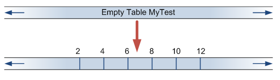
Now lets read a range:

SET TRANSACTION ISOLATION LEVEL SERIALIZABLE;
BEGIN TRAN
SELECT id FROM MyTest WHERE id BETWEEN 3 AND 8;
-- do concurrent stuff here.
COMMIT

illustration
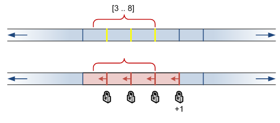
Books OnLine says: “The number of RangeS-S locks held is n+1, where n is the number of rows that satisfy the query.” We can verify this by looking at sys.dm_tran_locks. I’ve shown the locks that are taken above. Range locks apply to the range of possible values from the given key value, to the nearest key value below it.

You can see that the “locked range” of [2..10] is actually larger than the query range [3..8]. Attempts to insert rows into this range will wait.

What happens if we select a range containing all rows?

SET TRANSACTION ISOLATION LEVEL SERIALIZABLE;
BEGIN TRAN
SELECT id FROM MyTest WHERE id BETWEEN 1 AND 13;
-- do concurrent stuff here
COMMIT

illustration
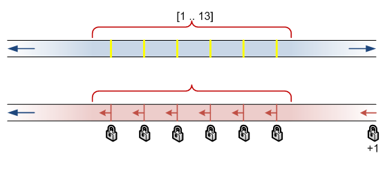
You can see that everything is selected. That lock at “infinity” has a resource_description value of (ffffffffffff).

Last interesting bit. Ghost records can participate in these ranges!

DELETE MyTest;
SET TRANSACTION ISOLATION LEVEL SERIALIZABLE;
BEGIN TRAN
SELECT id FROM MyTest WHERE id BETWEEN 1 AND 10;
-- do concurrent stuff here
COMMIT

illustration
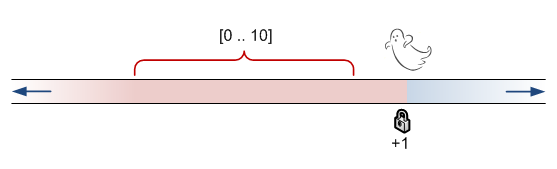
Concurrent transactions are able to insert values above 12, but will wait for values below that!

October 26, 2009

SQL Snippets is my new favourite thing.

Filed under: Miscelleaneous SQL — Tags: , , — Michael J. Swart @ 8:18 am

Within the last hour, Mladen Prajdić announced a new version of his popular SSMS Tools Pack version 1.7. The main new feature being SQL Snippets. This provides Management Studio an add-in that is very much like the code snippets in other IDEs everywhere.

Also within that last hour, I’ve installed and test-driven the new feature and it is officially my new favourite thing. I’ve got big plans for this feature. I’ve already translated my custom templates to it. In conjunction with templates (and Ctrl-Shift-M), I foresee great things for this feature.

Good job Mladen!

October 14, 2009

A Trick for Aggregating Data Fast

Filed under: Technical Articles — Tags: , , , — Michael J. Swart @ 5:49 pm

I want to explain a trick I came up with that helps an OLTP database do part of the job that OLAP cubes do. (Isn’t that cute, the database engine thinks it’s a cube.*)

If for some reason you find yourself wanting to use an OLTP database (i.e. regular old database) for something that is better suited to an OLAP cube (like Analysis Services for example) then you’re in good company! It seems to be a very common challenge. Even Microsoft seems to recognize this by implementing T-SQL tricks that step over the line into OLAP territory. Grouping sets comes to mind; Also another sign is that CUBE is now a keyword.

Aggregating Data Along a Dimension Before it’s Needed.
One task that is deep in the heart of OLAP territory is reporting the aggregate of a measurement along a dimension. I want to explain how to do this efficiently inside an OLTP db.

In the following examples the OLTP database (and wannabe OLAP cube) will be the standard AdventureWorks database. I’ll be using the Sales.SalesOrderDetail table. The measurement here is the LineTotal field, and the dimension here is the Product.

So we can report on this kind of data easily by maintaining statistics using an indexed view. (BTW, this is a great use-case for indexed views).

Here’s the trick. If n is the measurement, then the only stats we need to store are the sums of n0, n1, n2, grouped by the dimension. In other words, we keep track of the count, the sum and the sum of squares.

CREATE VIEW Sales.v_SalesOrderDetailAggregates WITH SCHEMABINDING
AS
SELECT ProductID,
   SUM(LineTotal) AS Sum1,
   COUNT_BIG(*) AS Count1,
   SUM(LineTotal*LineTotal) AS Sum2
FROM Sales.SalesOrderDetail
GROUP BY ProductID
GO
 
CREATE UNIQUE CLUSTERED INDEX IX_v_SalesOrderDetailAggregates
ON Sales.v_SalesOrderDetailAggregates(ProductID)
GO

Using the Indexed View

So that’s the clustered index I propose we create. As I’ll show later, this is enough. The work of aggregating the data is offloaded to the db. And the work is done once at creation and maintained automatically during any relevant transactions.

In the following code sample, I show how to use this view to report on many common stats (aggregates):

SET STATISTICS IO ON
 
-- a report that aggregates LineTotal over Products
SELECT
   ProductId,
   COUNT(LineTotal),
   SUM(LineTotal),
   AVG(LineTotal),
   STDEVP(LineTotal),
   STDEV(LineTotal),
   VARP(LineTotal),
   VAR(LineTotal)
FROM Sales.SalesOrderDetail
GROUP BY ProductID
ORDER BY ProductID
 
-- the same report (aggregate LineTotal over Products)
-- that uses the indexed view.
SELECT
   ProductID,
   [COUNT] = Count1,
   [SUM] = Sum1,
   [AVG] = Sum1 / Count1,
   [STDEVP] = 1.0/Count1 * SQRT(Count1*Sum2 - Sum1*Sum1),
   [STDEV] = 1.0/SQRT(Count1*(Count1-1)) * SQRT(Count1*Sum2 - Sum1*Sum1),
   [VARP] = (Sum2 - (Sum1*Sum1/Count1))/(Count1),
   [VAR] = (Sum2 - (Sum1*Sum1/Count1))/(Count1-1)
FROM Sales.v_SalesOrderDetailAggregates
WHERE Count1 > 1
ORDER BY ProductID
 
/*
results:
 
(266 row(s) affected)
Table 'SalesOrderDetail'. Scan count 1, logical reads 485, physical reads 0, read-ahead reads 0, lob logical reads 0, lob physical reads 0, lob read-ahead reads 0.
 
(266 row(s) affected)
Table 'v_SalesOrderDetailAggregates'. Scan count 1, logical reads 4, physical reads 0, read-ahead reads 0, lob logical reads 0, lob physical reads 0, lob read-ahead reads 0.
*/

So why not expand the indexed view to include everything from the beginning? Well, there are a couple problems with that. First is that you’ll get an error message like:

Msg 10125, Level 16, State 1, Line 2
Cannot create index on view "AdventureWorks.Sales.v_SalesOrderDetailAggregates" because it uses
aggregate "STDEV". Consider eliminating the aggregate, not indexing the view, or using alternate
aggregates. For example, for AVG substitute SUM and COUNT_BIG, or for COUNT, substitute
COUNT_BIG.

And so what I’ve shown here is that you can use a calculation involving COUNT_BIG, SUM(n) and SUM(n*n) to calculate common statistical aggregates like AVG, STDEV and VAR.

Besides, this strategy also takes the least space, and for a little extra work, you can aggregate on a grouping higher up in the dimension. That is, by using the entries in the index as subtotals in order to generate totals for larger groupings.

*– I’m probably missing an opportunity to include an awesome illustration for this post; something involving databases, cubes and square and round pegs.

October 4, 2009

Spotlight on Brad Schulz Y'all

Filed under: Miscelleaneous SQL — Tags: , , , , — Michael J. Swart @ 5:46 pm

Every now and then, I come across an idea where I think “Man, I wish I thought of that”

Reading Brad Shulz’s blog post The Age-Old SELECT * vs. SELECT 1 Debate was one of those times. In that blog post, he explains how relevant the select expressions are when used inside an EXISTS’s subquery. By looking at the official docs here: http://technet.microsoft.com/en-us/library/ms188336.aspx you’ll learn enough to get by. But after reading Brad Shulz’s article, you’ll never forget.

Brad is relatively new to SQL Server. He spent much of his career so far focused on Visual FoxPro and was a Visual Foxpro MVP for years. SQL Server is a new focus for him and he’s already moderating the MSDN T-SQL forum. It won’t be long before he’ll be able to create test database servers with one hand tied behind his back (Interesting trick: Sit on your right hand and try typing “create test database servers”.)

His blog http://bradsruminations.blogspot.com/ deserves more exposure. I was first introduced to the articles he writes in September as he syndicated his blog at SQLServerPedia.

His style is sometimes hilarious, and funny most of the time, but always clever. I’m always surprised when SQL Server writers manage to keep their articles engaging because of the subject matter. Brad seems to keep up just fine.

Also Must-Read (if only for the laughs)

Brad recently agreed to answer a number of questions I had. (Huge thanks Brad for taking the time!)

Michael J. Swart: What skills in Visual FoxPro (VFP) transfer easily to SQL Server? (Any surprising ones?)

Brad Schulz: Just working with the concepts of databases, tables, columns, relations, and indexes for many years in VFP makes the transfer easy.  And basic SQL syntax has been part of the VFP language since 1991, so that eliminates an enormous learning curve right away… We VFPers have been doing INSERT, UPDATE, DELETE, and SELECT for almost 20 years.

That being said, though, we would still do a lot of one-row-at-a-time processing, because it was easy and it was lightning fast.  But the equivalent of that in SQL (i.e. cursor) is slow as molasses, and I’ve learned a lot of set-based techniques in SQL Server that I had never used before.  Thank goodness that I started playing with T-SQL recently… I think I would have gone bananas if I had started with SQL2000 with no CROSS APPLY or CTE’s or window functions (i.e. the OVER clause).  How did you guys stay sane before SQL2005 came out?

Michael J. Swart: A common story is that many SQL Server professionals got their start as “accidental DBAs”. How did you get your start? Or how did you come to choose SQL Server as a focus?

Brad Schulz: My story’s not of the accidental variety.  I got a B.S. in Computer Science from USC (University of Southern California) in 1981.  I actually started out as a Building Design major, which is a combination of Architecture and Civil Engineering, but I dropped the Architecture class about a month into my freshman year, because I could see that I had no drawing talent whatsoever.  To fill that void, I ended up taking a FORTRAN class independent study with a Computer Science professor.  I gobbled it up, and finished the class in about 2 weeks.  The professor asked me to be a tutor for others taking the regular class.  I changed my major to Computer Science just before my sophomore year.

When I graduated from college, I immediately started working as a float in my parents’ pool.  But after a couple of months, a friend of the family recommended me to a pear-packing company in Kelseyville, California (I found out later they were the largest pear-packer in the state).  They had a computer system that no longer worked and the software company that custom wrote it for them was out of business.  To make a long story short, they hired me as a consultant (God knows why), and I read the manual on the programming language (a form of BASIC on an HP-250 machine) and ended up re-writing their entire system.  From that point, I got work by word-of-mouth, and I’ve been an independent developer ever since.

I worked in dBase II in the early 1980’s, and then eventually moved to dBase III, Quicksilver, Clipper, and then FoxBase+ and FoxPro.  I’ve found plenty of FoxPro work for more than 20 years, but it’s not going to last forever, so SQL Server seemed like the logical choice to move to.

Michael J. Swart: What motivates you to moderate the MSDN T-SQL Forum?

Brad Schulz: Back in the 1990’s I participated in the FoxForum on CompuServe, answering questions about FoxPro.  I enjoyed helping people, and I learned a lot just by helping others, and I learned new ideas from experts who hung out at the forum.  I wanted to duplicate that experience at the MSDN T-SQL Forum.  I’ve learned an incredible amount from some very talented people there.

Michael J. Swart: What motivates you to blog?

Brad Schulz: For one thing, I wanted to get myself known a little more in the SQL community.  Some of my blogs are humorous or tongue-in-cheek, and that’s just a release for the crazy creative side of me.  But I also enjoy writing “how-to” and “discovery” articles… they force me to practice and experiment more with T-SQL.  I wrote several articles for FoxTalk and FoxPro Advisor in the 1990’s, but the turnaround time took forever, from submission through the editing process, and then waiting months for eventual publication.  In contrast, I like the immediate publication of blog posts and getting immediate feedback.

Michael J. Swart: What’s one thing you can say about yourself that would make the SQL Server crowd say “Nifty”?

Brad Schulz: What’s a word that means “stylish; smart; fine; excellent” and rhymes with “thrifty”?  Okay, scratch that.

Let me see… I’m an adopted child whose birth-mother was German Catholic and who played the violin.  I always knew I was adopted.  My birth-mother had requested I be placed with a German Catholic family (which I was, though my mother was the Catholic and my father was the German).  My parents knew about the violin, and figured there was musical talent in me, so they set me up with piano lessons when I was 5.  I’ve been playing piano ever since (45 years).  The weird, spooky part is that I asked for more detailed non-identifying information from the adoption agency when I was about 25 years old, and when I received it, I was floored when it said that my birth-mother worked in and had a talent for “data processing” (whatever that meant in the 1950’s).  Talk about “nature” vs “nurture”… I think the “nature” argument wins hands-down!

I also have a passion for the stock market, which I discovered in 1998.  You can read more about that at my (now-on-hiatus) website http://www.stockciphering.com/whatis.htm.  The stock market is just one huge database of stocks and daily prices, isn’t it?  And so I wrote a suite of Visual FoxPro (VFP) programs to calculate technical analysis figures for stocks and produce buy signals for them, and I created the website to try to ca
pitalize on it.  The website never really set the world on fire, but in “eating my own dog food” and using the data for my own trading, I did very well… From Jan2003 to Mar2009, my IRA (where I do my trading) more than quadrupled in value, compared to the S&P500 which lost 25% of its value during that same period.

 Michael J. Swart: Thanks Brad

October 1, 2009

The ABCs of Management Studio Shortcuts

Filed under: Technical Articles — Tags: , , — Michael J. Swart @ 10:39 am

Today I was watching a webcast hosted by Brent Ozar and Tim Ford (congrats on the MVP awards guys). One topic came up was “which key do you press to execute a query in SSMS?.” F5 seemed to be the default key. However I found out that Ctrl+E did the same thing. This prompted me to enumerate the alphabet and to see what each shortcut combination accomplishes.

I’m also giving the shortcuts a rating from 0-5 based on how often I personally use them. 0 means never. 5 means I’d rather give up my spacebar than this shortcut.

BTW, I’m also not mentioning ALT keys, or SHIFT keys, that comes later. But first “CTRL, CTRL you must learn CTRL!”

Ctrl+A: Select all text (a standard text editor command) : 4
Ctrl+C: Copy (a standard text editor command) : 5
Ctrl+D: Show results in grid : 4
Ctrl+E: Execute (aka F5, aka Alt+X) : 0 but maybe that will improve now that I know about it.
Ctrl+F: Quick Find: 3
Ctrl+G: Goto line number: 0 I don’t use it, but then I don’t have line numbers turned on.
Ctrl+H: Quick Replace: 2
Ctrl+I: The best hidden treasure ever. Hit Ctrl+I and then type some text, you go straight to the next occurence of that string. Try it now, I’ll wait… Wasn’t that so cool? : 5
Ctrl+J: Intellisense’s list members (2008 only) : 3
Ctrl+K: First key of a two key shortcut that can help do lots of things. This is a doorway into cool stuff. : 3
Ctrl+L: Show execution plan. : 2
Ctrl+M: Include Actual Execution Plan : 2
Ctrl+N: New Query window with the same connection as the current one. : 2
Ctrl+O: Open file (pretty standard) : 3
Ctrl+P: Print (Still there for nostalgia purposes) : 0
Ctrl+R: Hide Results Pane : 4 A big help for screen real estate.
Ctrl+S: Save File : 3
Ctrl+T: Show results as text : 3
Ctrl+U: Puts focus on the choose database control (Mnemonic: U is for USE) : 4
Ctrl+V: Paste (a standard text editor command) : 5
Ctrl+X: Cut (a standard text editor command) : 4
Ctrl+Y: Redo (a standard text editor command) : 4
Ctrl+Z: Undo (a standard text editor command) : 4

So there you go, Seemingly still up for grabs is Ctrl+Q and Ctrl+B. These don’t appear to do anything.

September 28, 2009

Detecting Loops using Recursive CTEs

Filed under: SQL Scripts,Technical Articles — Tags: , , , , — Michael J. Swart @ 5:29 am

I want to write (for posterity) a solution to a problem I encountered last week. I was asked a question about the following error message:

The statement terminated. The maximum recursion 100 has
been exhausted before statement completion.

I was dealing with a table that represented a (0..*) to (0..*) relationship between objects I’ll call THINGS1:

CREATE TABLE PARENTS
(
   ParentId INT NOT NULL REFERENCES THING(Id),
   ChildId INT NOT NULL REFERENCES THING(Id),
   PRIMARY KEY (ParentId, ChildId)
)

We were attempting to populate a similar table called ANCESTORS using a recursive CTE. I suspected that the recursive CTE was not terminating because of a loop in the PARENTS table. That is to say, the data in the PARENTS table implied that some THING was its own ancestor. (Think of it this way, if you are your own parent, that also means you’re your own grandparent, great-grandparent etc…)

To help fix the data I needed to write a query that returned a list of all THINGs that were (somehow) their own ancestor. This is what I came up with. It’s inefficient, but it did the trick.

;WITH ANCESTORS_CTE
AS (
     SELECT ParentId AS AncestorId, ChildId AS DescendantId, 1  AS Depth
     FROM PARENTS
     UNION ALL
     SELECT ANCESTORS_CTE.AncestorId, PARENTS.ChildId, ANCESTORS_CTE.Depth + 1 AS Depth
     FROM ANCESTORS_CTE
     JOIN PARENTS
          ON ANCESTORS_CTE.DescendantId = PARENTS.ParentId
     WHERE ANCESTORS_CTE.Depth < 10
)
SELECT DISTINCT AncestorId
FROM ANCESTORS_CTE
WHERE AncestorId = DescendantId

1 Mathematically speaking, the PARENTS table represents the adjacency matrix of a directed acyclic graph.

September 25, 2009

CHAR: What is it Good For?

Filed under: Technical Articles — Tags: , , , , , , — Michael J. Swart @ 7:06 am

Takeaway: … Absolutely nothing (say it again).

What’s the difference between the CHAR datatype and the VARCHAR datatype? At the time of this writing Google gives thousands of web pages that are willing to explain the difference. Or if not explaining the difference at least explaining which is better and when. Here are two of the more interesting or important links:

What this Blogger Thinks
I’m going to put my vote with VARCHAR over CHAR in almost all circumstances. I’m going to list what I think are the stated benefits of CHAR and then hopefully show that the benefits are outweighed by consistency you get from applying VARCHAR as a rule of thumb always. (n.b. Throughout this post, the same arguments apply to NCHAR vs. NVARCHAR.)

Data Integrity:
Does SQL Server Complain if you give CHAR (10) less than ten characters?
At first glance, you might assume (the way I did) that the following benefit: That

CREATE TABLE example1 ( col CHAR (10) )

is somehow equivalent to

CREATE TABLE example2
(
    col VARCHAR (10),
    CHECK (LEN (col) = 10)
)

But it turns out not to be the case. Inserting strings shorter than ten characters into the column in example 1 does not produce an error. Instead, SQL Server pads the value with enough spaces to fill out the value of the column.

Size
And so we get to it. The main consideration when deciding between these types always seems to be size. VARCHAR as you know takes only the characters it needs, but it uses an extra two bytes to store the length of the string. That’s why Microsoft recommends using CHAR for strings that are going to be a consistent length.

So, I’ve decided to find out how much exactly. Using the sample database Adventureworks, I changed the tables that used NCHAR columns to identical tables that use NVARCHAR columns. And I found that the number of pages consumed was exactly the same (even after rebuilding indexes). I expected that though. The small savings you get in that case was not enough to be able to fit extra rows into a database page.

But here’s something that surprised me regarding null-able columns. If you are counting every byte, you’ll see that VARCHAR is the clear space saver when it comes to NULLS. You’ll find that CHAR (10) columns that are NULL still take ten bytes while VARCHAR (10) columns take zero bytes. This is another reason to pick VARCHAR over CHAR.

Semantics
What about semantically? When application developers sees a CHAR (10) column, it’s clear to them that data in the column is expected to be exactly 10 characters. This is a benefit to the CHAR data type.
It is not something that the VARCHAR data type conveys nicely. Even with a CHECK constraint or with documentation.

So I’ll concede that. Even though it’s possible to create user defined types that do something similar:

CREATE TYPE PostalCode FROM VARCHAR (6);
CREATE TYPE SIN FROM VARCHAR (9);
CREATE TYPE OneChar VARCHAR (1);

So are CHARS Completely Useless?
No, but I don’t see any real significant advantage either. And so I think it’s easier to apply VARCHAR as a rule of thumb and as a best practice without worrying about whether it’s better than CHAR. So pick VARCHAR and be done with it.

September 16, 2009

What the devil?

Filed under: Miscelleaneous SQL — Tags: , , — Michael J. Swart @ 8:59 pm

The devil you know vs. the devil you don’t.
A good friend of my told me about an issue she recently came across. It seems that a particular group of admins implemented SQL Server database mirroring in order to implement a kind of relatively cheap high availability solution. It’s a useful strategy that’s discussed in a number of places. Here and here for example. 

Well, something went wrong or I wouldn’t be writing right now. I’m not familiar with all of the details, but there was some wrinkles with the performance of the network and the database server became extremely slow. (despite what you might think, this really isn’t an article about database mirroring) It’s ironic that the very thing that was implemented to increase up-time was the cause of down-time.

From another perspective, this is a case of “The devil you know vs. The devil you don’t.” Here, they traded the devil they knew – that is, not having a warm standby server – with a devil they didn’t – in this case, production uptime now depended on network performance in an unexpected way.

Other examples of known vs. unknown devils:

  • Known bugs in version 1.0 vs. Unknown introduced bugs in version 2.0
  • Raid 0 vs. Misconfigured SANs
  • Reliability of municipal power vs. Possibly fawlty UPS systems
  • Add your own examples to the comments! (best two comments get a No-Prize – extra points for irony.)

I’ve actually witnessed the unknown devils above. And as a lover of irony, I smiled (tempered slightly by sympathy for those whose necks were on the line).

The devil is in the details
In the examples I’ve mentioned above, the unknown devils reared their heads because of exposure to an unforeseen risk. What can you do about it though? Well, what else is there to do? Get to know that unknown devil. Test, test, test with all the time and resources available to you. There really is no short-cut. And sometimes, with the right testing, if you’re thorough enough you can get it right…

God is in the details*
Getting it right means you get the high availability you were hoping for. The uninterupted power. Secure systems, the robust bug free software. Maybe even five nines.

I’ll leave you with one last devil you know vs. devil you don’t example. It’s a picture of me and my brother. Presumably you know me and not him. But which is the evil one? Increased difficulty: neither of us have a goatee. Unfair: the photos have been scrambled.

Who’s the evil one?

* — BTW, “God is in the details” is a quote by architect Mies van der Rohe. I’m in good company when quoting architects for this industry; you’ve heard of design patterns right?

September 10, 2009

View Blocked Process Reports using the Deadlock Graph Control

What am I looking at here?
Shown above is a set of blocked process report. But it’s being displayed using SQL Server’s Deadlock Graph Control. Here’s a detail of the graph:
I’m totally wearing my hacker hat with this. Microsoft built the deadlock graph control to display deadlock graphs generated by Microsoft’s tools. What I’ve done is to take a set of blocked process reports and reformat them to look like a deadlock graph. You can tell that it’s not a deadlock because the graph is a tree, with no cycles.
See that process with the X through it. Normally it indicates a deadlock victim. But in this case, I’ve repurposed the X to indicate the lead blocker (i.e. the stalled car in the traffic jam of blocked SQL Servers).
Why?
The graph is useful because it can tell a story graphically that would otherwise take maybe 100 times longer to understand by reading the xml reports directly.
A few years ago when I installed SQL Server 2005 for the first time, I played around with SQL Server profiler and traces in general and had one of those moments that made me say “nifty!” I was looking at a deadlock graph displayed graphically.
Not much later after that, I noticed that blocked process reports contain information very similar to deadlock graphs. It wasn’t much of a leap to think that with a little creative reformatting, I could make the deadlock graph control do something else useful with blocked process reports.
How?
So here’s what you do:
  1. Find a trace that contains blocked processes reports. If it’s not already, save it as a table called blocked. The script below assumes that a table called blocked has already been created. (Alternatively, create an synonym called blocked that refers to a table)
  2. Copy the script below and run it in Management Studio.
  3. Click the blocking chain xml of interest to you.
  4. Save the xml file as an xdl file.
  5. Close and reopen the file in Management Studio.
The man behind the curtains.
So here’s the script I talked about. It’s also an example of me flexing my XML muscles.

Update Mar. 29, 2010 Due to the size of the script and some other formatting issues, I’m providing the script as a link rather than something to copy and paste. Download the script here.

September 8, 2009

Finding the Lead Blocker in a Set of Blocked Process Reports

Traffic jam by lynac on FlickrTakeaway: Skip to the end for a script that reports the lead blocker for a set of Blocked Process Reports. And tune in later this week for a nifty graphing trick for blocked process chains.

On Blocking
Sometimes SQL Server is like a highway, and is prone to traffic jams. Blocking processes (not to be confused with deadlocked processes) are processes that are waiting for resources that are being used by other processes.

Every now and then people talk about blocking chains. These are blocked processes that are waiting in a line. Process A is waiting for Process B. Process B is waiting for Process C. etc… In all cases, you want to find the lead blocker (the head of the chain) and address any issues that that process has. Think of the traffic jam analogy, it’s no good trying to focus on the Toyota that’s waiting patiently; you have to focus on the stalled Honda in the front.

I can think of two good ways to analyze blocking and blocking chains. The first method analyzes the current state of the database. The other focuses on collected trace data:

Method 1: Look at the current state of the database:
Look at the DMVs that are available, or at least to the sys.processes table. These tables provide data about the current state of the database. These tables have been discussed by Tim Chapman here and by Kalen Delaney here (Kalen’s script was written before 2005 but is still awesome). Or in short, try a variety of other solutions found here: http://www.lmgtfy.com/?q=sql+blocking.chain. I’m not going to add another solution with this post.

Method 2: Look at Blocked process report events in a trace:
Another method of analyzing blocking chains looks at data that is retrieved in one or more Blocked processes report. These Blocked process reports are generated and captured using a server-side trace or by using SQL Profiler. The blocked process report holds a ton of useful information. You can find a good example here (courtesy Johnathan Kehayias): http://jmkehayias.blogspot.com/2008/09/monitoring-for-blocked-processes-on-sql.html

Notice that there are two xml nodes under the blocked-process-report tag. These two refer to two processes, a blocked process and a blocking process (always two there are, no more, no less). So what happens if you have a blocking chain involving 12 processes? Then you’ll have 11 events in your trace. 11 blocked process reports with the same timestamp. This can make it tricky to find the lead blocker (the stalled Honda).

One way is to scan through the trace to find the process that’s been blocked the longest (the blocked process report with the largest duration). The blocking process is likely to be the lead blocker.

Or you can use this script:

WITH rankedEvents AS
(
   SELECT ROW_NUMBER() OVER (PARTITION BY EndTime ORDER BY Duration DESC) AS myRank ,
       CAST (TEXTData AS XML) AS TEXTdata
   FROM blocked
   WHERE EventClass = 137
)
SELECT TEXTdata
FROM rankedevents
WHERE myRank = 1

where blocked is the name of the table where SQL trace data is stored.

Later this week I plan to describe a method where I use SQL Server’s Deadlock Graph control to display blocking chains.

Older Posts »

Powered by WordPress